Differential synthesis analysis with bakR and DESeq2

Introduction

Welcome! This vignette discusses how to perform differential synthesis analysis. It involves combining the output of bakR with that of a differential expression analysis software. The assumption is that at this point you have worked through the “Differential kinetic analysis with bakR” vignette, or its more succinct alternative. If that is not the case, I would highly suggest starting there and then coming back here once you’re familiar with the standard use cases of bakR.

These are the packages you are going to have to install and load in order to do everything presented in this vignette:

library(bakR)

# Packages that are NOT automatically installed when bakR is installed
library(DESeq2)
#> Loading required package: S4Vectors
#> Loading required package: stats4
#> Loading required package: BiocGenerics
#> 
#> Attaching package: 'BiocGenerics'
#> The following object is masked from 'package:bakR':
#> 
#>     plotMA
#> The following objects are masked from 'package:stats':
#> 
#>     IQR, mad, sd, var, xtabs
#> The following objects are masked from 'package:base':
#> 
#>     anyDuplicated, aperm, append, as.data.frame, basename, cbind,
#>     colnames, dirname, do.call, duplicated, eval, evalq, Filter, Find,
#>     get, grep, grepl, intersect, is.unsorted, lapply, Map, mapply,
#>     match, mget, order, paste, pmax, pmax.int, pmin, pmin.int,
#>     Position, rank, rbind, Reduce, rownames, sapply, setdiff, sort,
#>     table, tapply, union, unique, unsplit, which.max, which.min
#> 
#> Attaching package: 'S4Vectors'
#> The following object is masked from 'package:utils':
#> 
#>     findMatches
#> The following objects are masked from 'package:base':
#> 
#>     expand.grid, I, unname
#> Loading required package: IRanges
#> Loading required package: GenomicRanges
#> Loading required package: GenomeInfoDb
#> Loading required package: SummarizedExperiment
#> Loading required package: MatrixGenerics
#> Loading required package: matrixStats
#> 
#> Attaching package: 'MatrixGenerics'
#> The following objects are masked from 'package:matrixStats':
#> 
#>     colAlls, colAnyNAs, colAnys, colAvgsPerRowSet, colCollapse,
#>     colCounts, colCummaxs, colCummins, colCumprods, colCumsums,
#>     colDiffs, colIQRDiffs, colIQRs, colLogSumExps, colMadDiffs,
#>     colMads, colMaxs, colMeans2, colMedians, colMins, colOrderStats,
#>     colProds, colQuantiles, colRanges, colRanks, colSdDiffs, colSds,
#>     colSums2, colTabulates, colVarDiffs, colVars, colWeightedMads,
#>     colWeightedMeans, colWeightedMedians, colWeightedSds,
#>     colWeightedVars, rowAlls, rowAnyNAs, rowAnys, rowAvgsPerColSet,
#>     rowCollapse, rowCounts, rowCummaxs, rowCummins, rowCumprods,
#>     rowCumsums, rowDiffs, rowIQRDiffs, rowIQRs, rowLogSumExps,
#>     rowMadDiffs, rowMads, rowMaxs, rowMeans2, rowMedians, rowMins,
#>     rowOrderStats, rowProds, rowQuantiles, rowRanges, rowRanks,
#>     rowSdDiffs, rowSds, rowSums2, rowTabulates, rowVarDiffs, rowVars,
#>     rowWeightedMads, rowWeightedMeans, rowWeightedMedians,
#>     rowWeightedSds, rowWeightedVars
#> Loading required package: Biobase
#> Welcome to Bioconductor
#> 
#>     Vignettes contain introductory material; view with
#>     'browseVignettes()'. To cite Bioconductor, see
#>     'citation("Biobase")', and for packages 'citation("pkgname")'.
#> 
#> Attaching package: 'Biobase'
#> The following object is masked from 'package:MatrixGenerics':
#> 
#>     rowMedians
#> The following objects are masked from 'package:matrixStats':
#> 
#>     anyMissing, rowMedians

# Packages which are installed when bakR is installed
library(dplyr) 
#> 
#> Attaching package: 'dplyr'
#> The following object is masked from 'package:Biobase':
#> 
#>     combine
#> The following object is masked from 'package:matrixStats':
#> 
#>     count
#> The following objects are masked from 'package:GenomicRanges':
#> 
#>     intersect, setdiff, union
#> The following object is masked from 'package:GenomeInfoDb':
#> 
#>     intersect
#> The following objects are masked from 'package:IRanges':
#> 
#>     collapse, desc, intersect, setdiff, slice, union
#> The following objects are masked from 'package:S4Vectors':
#> 
#>     first, intersect, rename, setdiff, setequal, union
#> The following objects are masked from 'package:BiocGenerics':
#> 
#>     combine, intersect, setdiff, union
#> The following objects are masked from 'package:stats':
#> 
#>     filter, lag
#> The following objects are masked from 'package:base':
#> 
#>     intersect, setdiff, setequal, union
library(magrittr) 
#> 
#> Attaching package: 'magrittr'
#> The following object is masked from 'package:GenomicRanges':
#> 
#>     subtract
library(ggplot2) 
library(stats)

# Set the seed for reproducibility
set.seed(123)

Intro to differential synthesis analysis

I claim that bakR is a tool for performing differential kinetic analysis, but if you are coming from the “Differential kinetic analysis with bakR” vignette then you might think that this is a misnomer. All that I showed you how to do in that vignette was differential stability analysis. Full-fledged differential kinetic analysis means performing differential synthesis analysis as well, so let’s talk about how you can do that with bakR.

bakR won’t be able to accomplish this task alone. The reason for this is that assessing changes in synthesis means assessing changes in RNA stability and RNA expression. Therefore, we need to perform differential expression analysis in conjunction with differential stability analysis. In theory, I could have implemented my own differential expression analysis in bakR, but with so many popular software tools currently in existence to perform that task, it seemed pointlessly redundant. It also gives you the freedom to use whatever differential expression analysis tool that you are used to using, and to perform whatever kind of DE analysis that you like independent of bakR.

Differential synthesis rate analysis with bakR + DESeq2

To show you how to perform differential synthesis analysis, I will be using DESeq2 for the purpose of differential expression analysis. Why? Because I like DESeq2. It’s a nice model, it’s a good piece of software, and it was an early source of inspiration for me in my PhD. Also, you’ll see that some of the output of bakR is specifically designed with DESeq2 in mind, so it will facilitate the process of performing differential expression analysis a bit.

First things first, let’s simulate some data! We’ll simulate 1000 genes, with 200 observing differential synthesis and no changes in stability. Let’s also run the efficient bakR implementation while we are at it.

# Simulate a nucleotide recoding dataset
sim_data <- Simulate_bakRData(1000,
                         num_kd_DE = c(0, 0),
                         num_ks_DE = c(0, 200))
  # This will simulate 500 features, 2 experimental conditions
  # and 3 replicates for each experimental condition
  # See ?Simulate_bakRData for details regarding tunable parameters

# Extract simulated bakRData object
bakRData <- sim_data$bakRData

# Extract simualted ground truths
sim_truth <- sim_data$sim_list

## Run the efficient model
# We'll tell it what the mutation rates are just for efficiency's sake
Fit <- bakRFit(bakRData, pnew = rep(0.05, times = 6), pold = 0.001)
#> Finding reliable Features
#> Filtering out unwanted or unreliable features
#> Processing data...
#> Using provided pnew estimates
#> Using provided pold estimate
#> Estimated pnews and polds for each sample are:
#>   mut reps pnew  pold
#> 1   1    1 0.05 0.001
#> 2   1    2 0.05 0.001
#> 3   1    3 0.05 0.001
#> 4   2    1 0.05 0.001
#> 5   2    2 0.05 0.001
#> 6   2    3 0.05 0.001
#> Estimating fraction labeled
#> Estimating per replicate uncertainties
#> Estimating read count-variance relationship
#> Averaging replicate data and regularizing estimates
#> Assessing statistical significance
#> All done! Run QC_checks() on your bakRFit object to assess the 
#>             quality of your data and get recommendations for next steps.

The second step is to perform differential expression analysis. As I alluded to above, bakR makes this a bit easier, and the way it does that is by providing a count matrix formatted just how DESeq2 likes it! DESeq2 also requires one more input, and that is a dataframe that provides information about any covariates (things that distinguish samples). Here is all the code to produce those necessary inputs


# Get the count matrix from bakR
Counts <- Fit$Data_lists$Count_Matrix

# Experimental conditions for each sample
# There are 6 s4U treated samples (3 replicates of each condition)
# In addition, there are 2 -s4U control samples (1 for each condition)

## s4U conditions
# 1st three samples are reference (ref) samples
# Next three samples are experimental (exp) samples
conditions_s4U <- as.factor(rep(c("ref", "exp"), each = 3))

## -s4U control conditions
# 1st sample is reference, next is experimental
conditions_ctl <- as.factor(c("ref", "exp"))

# Combined s4U and -s4U control conditions
conditions <- c(conditions_s4U, conditions_ctl)

# Make the colData input for DESeq2
colData <- data.frame(conditions = conditions)
rownames(colData) <- colnames(Counts)

# Take a look at the colData object
print(t(colData))

	1	2	3	4	5	6	7	8
conditions	ref	ref	ref	exp	exp	exp	ref	exp

Once you make sure that you have correctly mapped samples to experimental conditions in the colData object, you can create that sweet sweet DESeqDataObject

dds <- DESeqDataSetFromMatrix(countData = Counts,
                              colData = colData,
                              design = ~conditions)
#> converting counts to integer mode

I invite you to read the DESeq2 documentation if you need help understanding the call to DESeqDataSetFromMatrix. In short though, the first entry is our count matrix, the second is our colData object, and the final entry is the design matrix. Limma’s documentation (another differential expression analysis software) has a great introduction to design matrices, but this one is simple. It means that we want to group samples together that have the same value for the conditions factor in the colData object. So all “ref” samples will be grouped together and all “exp” samples will be grouped together. DESeq2 will then compare different groups, which means that it will compare “exp” and “ref” samples in this case.

Now we can fit DESeq2 and extract the differential expression analysis results:

ddso <- DESeq(dds)
#> estimating size factors
#> estimating dispersions
#> gene-wise dispersion estimates
#> mean-dispersion relationship
#> final dispersion estimates
#> fitting model and testing

# Extract results of experimental vs. reference comparison
reso <- results(ddso, contrast = c("conditions", "exp", "ref"))

# Look at the column names of the reso object
colnames(as.data.frame(reso))
#> [1] "baseMean"       "log2FoldChange" "lfcSE"          "stat"          
#> [5] "pvalue"         "padj"

For our sake, we are going to use two columns in the reso object: log2FoldChange and lfcSE. Both of these column names are pretty self-explanatory, but for completeness sake, log2FoldChange is the log base-2 fold change in RNA expression, and lfcSE is the standard error in the log2FoldChange.

With that, we have all we need to perform differential synthesis analysis! But how you may ask? Well, if our population of cells that we performed RNA-seq on was at steady-state (i.e., the cells were not actively responding to some perturbation while treating with with a metabolic label), then the following relationship holds between \(ksyn\) (RNA synthesis rate) \(kdeg\) (RNA degradation rate) and \([RNA]\) (RNA concentration):

\[ [RNA] = \frac{ksyn}{kdeg} \]

Therefore, the log2 fold change in \([RNA]\) (\(L2FC(RNA)\)) is: \[ \begin{align} L2FC(RNA) &= log_2(\frac{[RNA_{exp}]}{[RNA_{ref}]}) \\ &= log_2(\frac{ksyn_{exp}*kdeg_{ref}}{ksyn_{ref}*kdeg_{exp}}) \\ &= log_2(\frac{ksyn_{exp}}{ksyn_{ref}}) - log_2(\frac{kdeg_{exp}}{kdeg_{ref}}) \\ &= L2FC(ksyn) - L2FC(kdeg) \end{align} \] Therefore, the key conclusion for performing differential synthesis analysis is that:

\[ L2FC(ksyn) = L2FC(RNA) + L2FC(kdeg) \]

bakR provides \(L2FC(kdeg)\) and DESeq2 provides \(L2FC(RNA)\), so we have everything we need to calculate the \(L2FC(ksyn)\). Let’s make a data.frame with this information:

ksyn_df <- data.frame(L2FC = reso$log2FoldChange + Fit$Fast_Fit$Effects_df$L2FC_kdeg,
                      Gene = Fit$Fast_Fit$Effects_df$XF)

We are missing one key component though: the uncertainty (or standard error). How can we get that from bakR and DESeq2? Well the easiest and most conservative thing to do is to assume independence of \(L2FC(RNA)\) and \(L2FC(kdeg)\). That’s because the variances of independent random variables add, so that:

\[ \begin{align} \text{Var}[L2FC(ksyn)] &= \text{Var}[L2FC(kdeg) + L2FC(RNA)] \\ &= \text{Var}[L2FC(kdeg)] + \text{Var}[L2FC(RNA)] \end{align} \]

where \(\text{Var}[X]\) is the variance of random variable \(X\). We can then calculate the standard error as the square root of the variance, meaning:

\[ \text{se}[L2FC(ksyn)] = \sqrt{se[L2FC(kdeg)]^2 + se[L2FC(RNA)]^2} \] where I am using the non-standard notation \(\text{se}[X]\) to mean the standard error of \(X\). With this, we can fill out the final component of the L2FC(ksyn) dataframe:

ksyn_df$se <- sqrt(reso$lfcSE^2 + (Fit$Fast_Fit$Effects_df$se*log2(exp(1)))^2 )

The se in Effects_df is for the log base-e fold change in \(kdeg\), so we have to use the fact that:

\[ \text{Var}[a*X] = a^2*\text{Var}[X] \] for some constant a. In this case, a is \(log_2(e)\) because that is the multiplicative factor necessary to convert from log base-2 to log base-e. Now all that is left is to calculate the p-value and multiple-test adjust it (I am going to use Benjamini-Hochberg for multiple test adjustment because that is what both bakR and DESeq2 use).

# Calculate p-value using asymptotic Wald test
ksyn_df <- ksyn_df %>%
  mutate(pval = 2*pnorm(-abs(L2FC/se)),
         padj = p.adjust(pval, method = "BH"))

You can now make a \(L2FC(ksyn)\) volcano plot to visualize the final conclusions!


# Add conclusion at 0.01 FDR control
ksyn_df <- ksyn_df %>%
  mutate(conclusion = as.factor(ifelse(padj < 0.01, 
                             ifelse(L2FC < 0, "Decreased txn", "Increased txn"),
                             "Not sig.")))

# Make volcano plot
ksyn_volc <- ggplot(ksyn_df, aes(x = L2FC, y = -log10(padj), color = conclusion)) + 
  theme_classic() + 
  geom_point(size = 1) + 
  xlab("L2FC(ksyn)") + 
  ylab("-log10(padj)") + 
  scale_color_manual(values = c("blue", "orange", "gray"))

# Observe volcano plot
ksyn_volc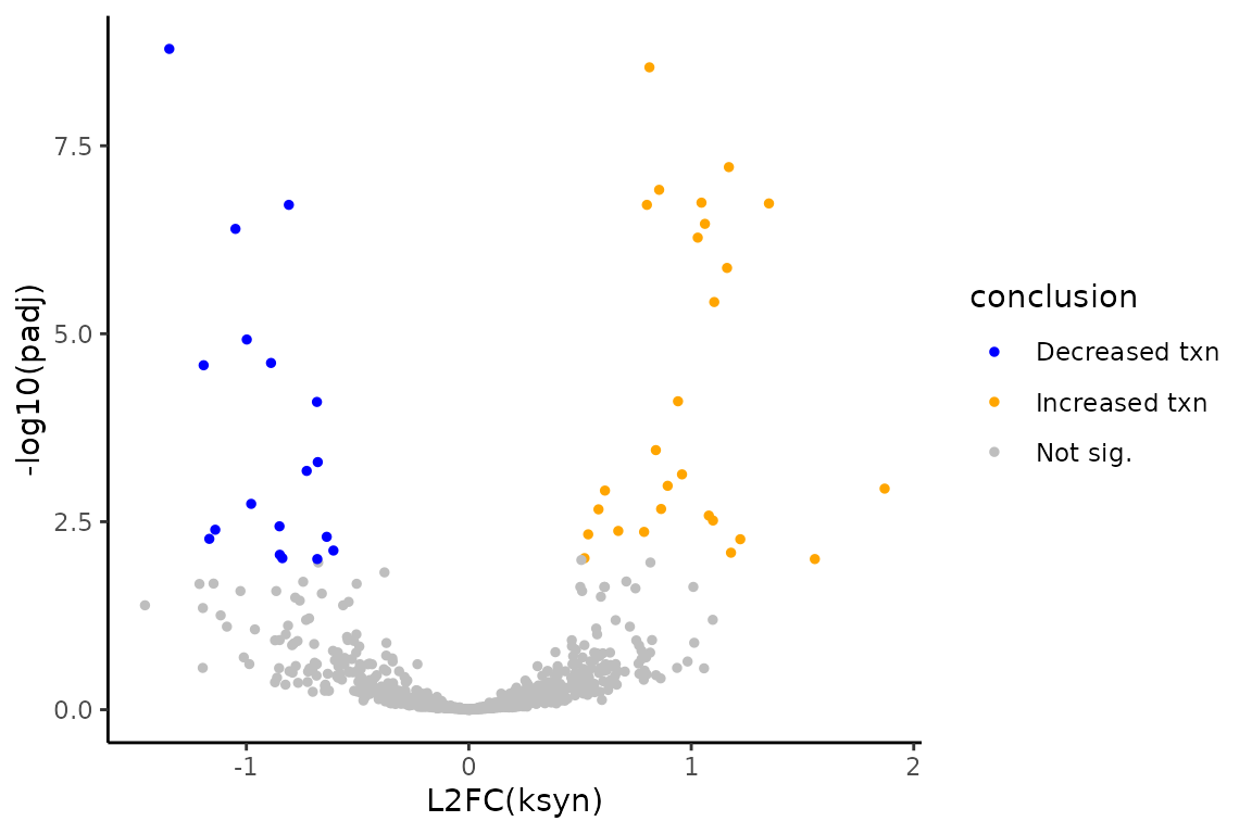

The simulation is such that features number 1-800 will be the non-differentially synthesized RNA and features 801-1000 will be the 200 differentially synthesized RNA. Therefore, we can also see how the analysis performed


# Add conclusion at 0.01 FDR control
ksyn_df <- ksyn_df %>%
  mutate(result = as.factor(ifelse(padj < 0.01, 
                             ifelse(as.integer(Gene) <= 800, "FP", "TP"),
                             ifelse(as.integer(Gene) <= 800, "TN", "FN"))))

# Make volcano plot
ksyn_results <- ggplot(ksyn_df, aes(x = L2FC, y = -log10(padj), color = result)) + 
  theme_classic() + 
  geom_point(size = 1) + 
  xlab("L2FC(ksyn)") + 
  ylab("-log10(padj)") + 
  scale_color_manual(values = c("black", "gray", "forestgreen", "blue"))

# Observe volcano plot
ksyn_results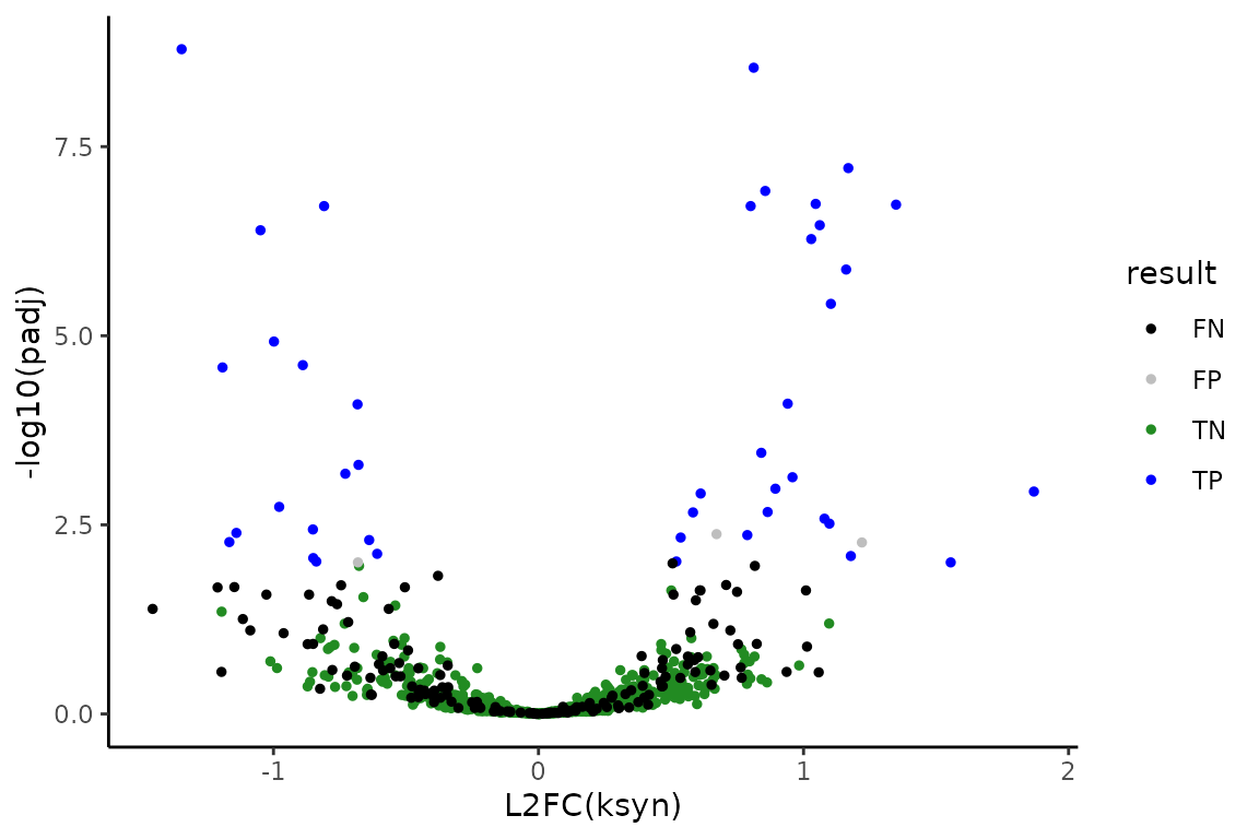

FP is a false positive, FN is a false negative, TP is a true positive, and TN is a true negative. All in all, I’d say it went pretty well! You now know how to perform differential synthesis analysis with bakR + DEseq2.

NOTE: As of version 1.0.0 of bakR, DissectMechanism is a function in bakR that will implement this analysis strategy for you. See the vignette on mechanistic dissection for more details.

Isaac Vock

Introduction

Intro to differential synthesis analysis

Differential synthesis rate analysis with bakR + DESeq2