Correcting for dropout

Abstract

Dropout is the phenomenon by which metabolically labeled RNA or sequencing reads derived from such RNA is lost either during library preparation or during computational processing of the raw sequencing data. Several labs have independently identified and discussed the prevalence of dropout in NR-seq and other metabolic labeling RNA-seq experiments. Recent work suggests that there are three potential causes for this: 1) Loss of labeled RNA on plastic surfaces during RNA extraction, 2) RT falloff due to modifications of the metabolic labeling made by some NR-seq chemistries, and 3) loss of reads with many NR-induced mutations due to poor read alignment. While 3) is best remedied by improved alignment strategies (discussed in Zimmer et al. and Berg et al.), modified fastq processing will not address the other causes. Improved handling of RNA can help, but what if you already have data that you suspect may be biased by dropout? Version 1.0.0 of bakR introduced a strategy to correct for dropout induced biases. In this vignette, I will show how to correct for dropout with bakR. Following the demonstrations, I will also include a more thorough discussion of dropout, bakR’s dropout correction strategy, and how it differs from a strategy recently developed by the Erhard lab.

Necessary Setup

bakR version 1.0.0 or later is necessary to run this vignette.

library(bakR)
set.seed(123)

A Brief Tutorial on Dropout Correction in bakR

bakR has a new simulation strategy as of version 1.0.0 that allows for the accurate simulation of dropout:

# Simulate a nucleotide recoding dataset
sim_data <- Simulate_relative_bakRData(1000, depth = 1000000, nreps = 2,
                                       p_do = 0.4)
  # This will simulate 500 features, 500,000 reads, 2 experimental conditions
  # and 2 replicates for each experimental condition.
  # 40% dropout is simulated.
  # See ?Simulate_relative_bakRData for details regarding tunable parameters

# Run the efficient model
Fit <- bakRFit(sim_data$bakRData)
#> Finding reliable Features
#> Filtering out unwanted or unreliable features
#> Processing data...
#> Estimating pnew with likelihood maximization
#> Estimating unlabeled mutation rate with -s4U data
#> Estimated pnews and polds for each sample are:
#> # A tibble: 4 × 4
#> # Groups:   mut [2]
#>     mut  reps   pnew    pold
#>   <int> <dbl>  <dbl>   <dbl>
#> 1     1     1 0.0497 0.00100
#> 2     1     2 0.0500 0.00100
#> 3     2     1 0.0499 0.00100
#> 4     2     2 0.0497 0.00100
#> Estimating fraction labeled
#> Estimating per replicate uncertainties
#> Estimating read count-variance relationship
#> Averaging replicate data and regularizing estimates
#> Assessing statistical significance
#> All done! Run QC_checks() on your bakRFit object to assess the 
#>             quality of your data and get recommendations for next steps.

Dropout will cause bakR to underestimate the true fraction new. In addition, low fraction new features will receive more read counts than they would have if dropout had not existed (and vice versa for high fraction new features). Both of these biases can be corrected for with a single line of code:

# Correct dropout-induced biases
Fit_c <- CorrectDropout(Fit)
#> Estimated rates of dropout are:
#>   Exp_ID Replicate       pdo
#> 1      1         1 0.4013715
#> 2      1         2 0.3841179
#> 3      2         1 0.2627656
#> 4      2         2 0.3242958
#> Mapping sample name to sample characteristics
#> Filtering out low coverage features
#> Processing data...
#> Estimating read count-variance relationship
#> Averaging replicate data and regularizing estimates
#> Assessing statistical significance
#> All done! Run QC_checks() on your bakRFit object to assess the 
#>             quality of your data and get recommendations for next steps.
  # You can also overwite the existing bakRFit object.
  # I am creating a separate bakRFit object to make comparisons later in this vignette.

Dropout will lead to a correlation between the fraction new and the difference between +s⁴U and -s⁴U read counts. This trend and the model fit can be visualized as follows:

# Correct dropout-induced biases
Vis_DO <- VisualizeDropout(Fit)
#> Estimated rates of dropout are:
#>   Exp_ID Replicate       pdo
#> 1      1         1 0.4013715
#> 2      1         2 0.3841179
#> 3      2         1 0.2627656
#> 4      2         2 0.3242958

# Visualize dropout for 1st replicate of reference condition
Vis_DO$ExpID_1_Rep_1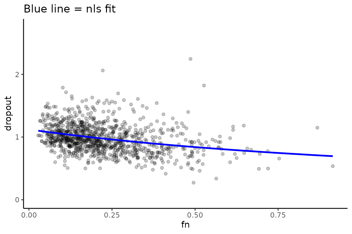

We can assess the impact of dropout correction by comparing the known simulated truth to the fraction new estimates, before and after dropout correction.

Before correction:


# Extract simualted ground truths
sim_truth <- sim_data$sim_list

# Features that made it past filtering
XFs <- unique(Fit$Fast_Fit$Effects_df$XF)

# Simulated logit(fraction news) from features making it past filtering
true_fn <- sim_truth$Fn_rep_sim$Logit_fn[sim_truth$Fn_rep_sim$Feature_ID %in% XFs]

# Estimated logit(fraction news)
est_fn <- Fit$Fast_Fit$Fn_Estimates$logit_fn

# Compare estimate to truth
plot(true_fn, est_fn, xlab = "True logit(fn)", ylab = "Estimated logit(fn)")
abline(0, 1, col = "red")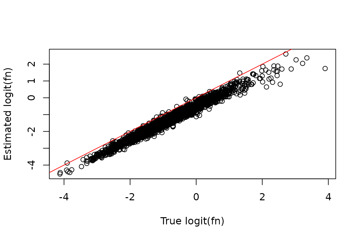

After correction:


# Features that made it past filtering
XFs <- unique(Fit_c$Fast_Fit$Effects_df$XF)

# Simulated logit(fraction news) from features making it past filtering
true_fn <- sim_truth$Fn_rep_sim$Logit_fn[sim_truth$Fn_rep_sim$Feature_ID %in% XFs]

# Estimated logit(fraction news)
est_fn <- Fit_c$Fast_Fit$Fn_Estimates$logit_fn

# Compare estimate to truth
plot(true_fn, est_fn, xlab = "True logit(fn)", ylab = "Estimated logit(fn)")
abline(0, 1, col = "red")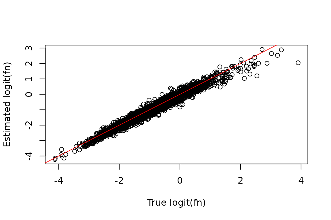

RNA dropout and bakR’s correction strategy

As discussed in the Abstract for this vignette, dropout refers to the loss of metabolically labeled RNA, or reads from said RNA. Dropout correction in the context of bakR is specifically designed to address biases due to the loss of metabolically labeled RNA during library preparation.

bakR’s strategy for correcting dropout involves formalizing a model for dropout, using that model to infer a parametric relationship between the biased fraction new estimate and the ratio of +s⁴U to -s⁴U read counts for a feature, and then fitting that model to data with nonlinear least squares. bakR’s model of dropout makes several simplifying assumptions to ensure tractability of parameter estimation while still capturing important features of the process:

The average number of reads that will come from an RNA feature is related to the fraction of sequenced RNA molecules derived from that feature.
All labeled RNA is equally likely to get lost during library preparation, with the probability of losing a molecule of labeled RNA referred to as pdo.

These assumptions lead to the following expressions for the expected number of sequencing reads coming from a feature (index i) in +s⁴U and -s⁴U NR-seq data:

\[ \begin{align} \text{E[reads from feature i in +s}^{\text{4}}\text{U sample]} &= \frac{\text{number of molecules from feature i}}{\text{total number of molecules in +s}^{\text{4}}\text{U sample}}*\text{R}_{\text{+s}^{\text{4}}\text{U}} \\ &= \frac{\text{n}_{\text{i}}*\theta_{\text{i}}*(1 - \text{pdo}) + \text{n}_{\text{i}}*(1 - \theta_{\text{i}}) }{\sum_{\text{j}=1}^{\text{NF}}\text{n}_{\text{j}}*\theta_{\text{j}}*(1 - \text{pdo}) + \text{n}_{\text{j}}*(1 - \theta_{\text{j}}) }*\text{R}_{\text{+s}^{\text{4}}\text{U}} \\ \\ \\ \text{E[reads from feature i in -s}^{\text{4}}\text{U sample]} &= \frac{\text{number of molecules from feature i}}{\text{total number of molecules in -s}^{\text{4}}\text{U sample}}*\text{R}_{\text{-s}^{\text{4}}\text{U}} \\ &= \frac{\text{n}_{\text{i}}}{\sum_{\text{j}=1}^{\text{NF}}\text{n}_{\text{j}}}*\text{R}_{\text{-s}^{\text{4}}\text{U}} \end{align} \]

where the parameters are defined as follows:

\[ \begin{align} \text{n}_{\text{i}} &= \text{Number of molecules from feature i} \\ \theta_{\text{i}} &= \text{True fraction new for feature i} \\ \text{pdo} &= \text{Probability that a labeled RNA molecule is preferentially lost during library prep} \\ \text{NF} &= \text{Total number of RNA features that contribute sequencable molecules} \\ \text{R} &= \text{Total number of sequencing reads.} \end{align} \]

Defining “dropout” to be the ratio of the RPM normalized expected read counts yields the following relationship between “dropout”, the fraction new, and the rate of dropout:

\[ \begin{align} \text{Dropout} &= \frac{\text{E[reads from feature i in +s}^{\text{4}}\text{U sample]/}\text{R}_{\text{+s}^{\text{4}}\text{U}}}{\text{E[reads from feature i in -s}^{\text{4}}\text{U sample]/}\text{R}_{\text{-s}^{\text{4}}\text{U}}} \\ \\ &= \frac{\text{n}_{\text{i}}*\theta_{\text{i}}*(1 - \text{pdo}) + \text{n}_{\text{i}}*(1 - \theta_{\text{i}}) }{\text{n}_{\text{i}}}*\frac{\sum_{\text{j}=1}^{\text{NF}}\text{n}_{\text{j}}}{ \sum_{\text{j}=1}^{\text{NF}}\text{n}_{\text{j}}*\theta_{\text{j}}*(1 - \text{pdo}) + \text{n}_{\text{j}}*(1 - \theta_{\text{j}}) } \\ \\ &= [\theta_{\text{i}}*(1 - \text{pdo}) + (1 - \theta_{\text{i}})]*\text{scale} \\ &= [1 - \theta_{\text{i}}*\text{pdo}]*\text{scale} \end{align} \]

where \(\text{scale}\) is a constant scale factor that represents the factor difference in the number of sequencable molecules with and without dropout.

Currently, the relationship between the quantification of dropout and \(\text{pdo}\) includes \(\theta_{\text{i}}\), which is the true, unbiased fraction new. Unfortunately, the presence of dropout means that we do not have access to this quantify. Rather, we estimate a dropout biased fraction of sequencing reads that are new (\(\theta_{\text{i}}^{\text{do}}\)), which on average will represent an underestimation of \(\theta_{\text{i}}\). Therefore, we need to relate the quantity we estimate (\(\theta_{\text{i}}^{\text{do}}\)) and the parameter we wish to estimate (\(\text{pdo}\)) to \(\theta_{\text{i}}\). In the context of this model, such a relationship can be derived as follows:

\[ \begin{align} \theta_{\text{i}}^{\text{do}} &= \frac{\text{number of new sequencable molecules}}{\text{total number of sequencable molecules}} \\ \theta_{\text{i}}^{\text{do}} &= \frac{\text{n}_{\text{i}}*\theta_{\text{i}}*(1 - \text{pdo}) }{\text{n}_{\text{i}}*\theta_{\text{i}}*(1 - \text{pdo}) + \text{n}_{\text{i}}*(1-\theta_{\text{i}})} \\ \theta_{\text{i}}^{\text{do}} &= \frac{\theta_{\text{i}}*(1 - \text{pdo}) }{\theta_{\text{i}}*(1 - \text{pdo}) + (1-\theta_{\text{i}})} \\ \theta_{\text{i}}^{\text{do}}*[1 - \theta_{\text{i}}*\text{pdo}] &= \theta_{\text{i}}*(1 - \text{pdo}) \\ \theta_{\text{i}}^{\text{do}} &= \theta_{\text{i}}*(1 - \text{pdo}) + \theta_{\text{i}}*\theta_{\text{i}}^{\text{do}}*\text{pdo} \\ \frac{\theta_{\text{i}}^{\text{do}}}{(1 - \text{pdo}) + \theta_{\text{i}}^{\text{do}}*\text{pdo}} &= \theta_{\text{i}} \end{align} \]

We can then use this relationship to substite \(\theta_{\text{i}}\) for a function of \(\theta_{\text{i}}^{\text{do}}\) and \(\text{pdo}\) in our dropout quantification equation:

\[ \begin{align} \text{Dropout} &= [1 - \theta_{\text{i}}*\text{pdo}]*\text{scale}\\ \text{Dropout} &= \text{scale} - \frac{\text{scale}*\text{pdo}*\theta_{\text{i}}^{\text{do}}}{(1 - \text{pdo}) + \theta_{\text{i}}^{\text{do}}*\text{pdo}} \end{align} \]

bakR’s CorrectDropout function fits this predicted relationship between the ratio of +s⁴U to -s⁴U reads (\(\text{Dropout}\)) and the uncorrected fraction new estimates (\(\theta_{\text{i}}^{\text{do}}\)) to infer \(pdo\). Corrected fraction new estimates can then be inferred from the relationship between \(\theta_{\text{i}}^{\text{do}}\), \(\text{pdo}\), and \(\theta_{\text{i}}\). Finally, bakR redistributes read counts according to what the estimated relative proportions of each feature would have been if no dropout had existed. The key insight is that:

\[ \begin{align} \frac{\text{E[number of reads without dropout]}}{\text{E[number of reads with dropout]}} &= \text{Dropout}\\ &= \frac{\text{n}_{\text{i}}*\theta_{\text{i}}*(1 - \text{pdo}) + \text{n}_{\text{i}}*(1 - \theta_{\text{i}}) }{\text{n}_{\text{i}}}*\frac{\sum_{\text{j}=1}^{\text{NF}}\text{n}_{\text{j}}}{ \sum_{\text{j}=1}^{\text{NF}}\text{n}_{\text{j}}*\theta_{\text{j}}*(1 - \text{pdo}) + \text{n}_{\text{j}}*(1 - \theta_{\text{j}}) } \\ &= \frac{\theta_{\text{i}}*(1 - \text{pdo}) + (1 - \theta_{\text{i}}) }{1}*\frac{\text{N}}{\text{N}*\theta_{\text{G}}*(1-\text{pdo}) + \text{N}*(1 - \theta_{\text{G}})}\\ &= \frac{\theta_{\text{i}}*(1 - \text{pdo}) + (1 - \theta_{\text{i}}) }{1}*\frac{1}{\theta_{\text{G}}*(1 - \text{pdo}) + (1 - \theta_{\text{G}}) } \\ \\ &= \frac{\text{fraction of feature i molecules remaining after dropout}}{\text{fraction of total molecules remaining after dropout}} \\ \end{align} \]

Getting from the 2nd line to the third line involved a bit of algebraic trickery (multiplying by 1) and defining the “global fraction new” (\(\theta_{\text{G}}\)), which is the fraction of all sequenced molecules that are new (where \(\text{N}\) is the total number of sequenced molecules if none are lost due to dropout). \(\theta_{\text{G}}\) can be calculated as a weighted average of dropout biased fraction news for each feature, weighted by the uncorrected number of reads each feature has, and then dropout correcting:

\[ \begin{align} \theta_{\text{G}}^{\text{do}} &= \frac{\sum_{\text{j=1}}^{\text{NF}}\theta_{\text{j}}^{\text{do}}*\text{nreads}_{\text{j}} }{\sum_{\text{j=1}}^{\text{NF}}\text{nreads}_{\text{j}}} \\ \theta_{\text{G}} &= \frac{\theta_{\text{G}}^{\text{do}}}{(1 - \text{pdo}) + \theta_{\text{G}}^{\text{do}}*\text{pdo}} \end{align} \]

Thus, the dropout corrected read counts can be obtained as follows:

\[ \begin{align} \text{Corrected read count for feature i} &= \text{nreads}_{\text{i}}*\frac{\theta_{\text{i}}*(1 - \text{pdo}) + (1 - \theta_{\text{i}})}{\theta_{\text{G}}*(1 - \text{pdo}) + (1 - \theta_{\text{G}})} \end{align} \]

Differences between bakR and grandR’s strategies

Florian Erhard’s group was the first to implement a strategy for dropout correction in an NR-seq analysis tool (their R package grandR). The strategy used by grandR is discussed here. In short, the dropout rate (\(\text{pdo}\)) is assumed to be related to the Spearman correlation (\(\rho\)) between the rank of a feature’s fraction new(referred to by them as the new-to-total ratio, or NTR) and the log of the dropout metric discussed above (ratio of +s⁴U to -s⁴U read counts) as follows:

\[ \begin{align} \text{pdo} &= \frac{\rho}{\rho + 1} \end{align} \]

We note that this definition is not model derived and sets an artificial upper bound on \(\text{pdo}\) of 0.5. The estimated number of sequencing reads from new RNA is then multiplied by a factor (\(\text{f}\)) defined as follows:

\[ \text{f} = \frac{1}{1 - \text{pdo}} \]

and the corrected fraction new is estimated using the adjusted new RNA read counts. A bit of algebra shows that this relationship between the inferred \(\text{pdo}\) and the corrected fraction new is identical to that derived from the model above:

\[ \begin{align} \theta_{\text{i}} &= \frac{\text{f}*(\text{number of reads from new RNA})}{\text{f}*(\text{number of reads from new RNA}) + (\text{number of reads from old RNA})} \\ &= \frac{\text{f}*\theta_{\text{i}}^{\text{do}}*\text{nreads}_{\text{i}}}{\text{f}*\theta_{\text{i}}^{\text{do}}*\text{nreads}_{\text{i}} + (1 - \theta_{\text{i}}^{\text{do}})*\text{nreads}_{\text{i}}} \\ &= \frac{\frac{\theta_{\text{i}}^{\text{do}}}{(1 - \text{pdo})}}{\frac{\theta_{\text{i}}^{\text{do}}}{(1 - \text{pdo})} + (1 - \theta_{\text{i}}^{\text{do}})} \\ &= \frac{\theta_{\text{i}}^{\text{do}}}{(1 - \text{pdo}) + \theta_{\text{i}}^{\text{do}}*\text{pdo}} \end{align} \]

Thus, grandR is implicitly making assumptions similar to those laid out in the model above that is used by bakR.

Notable differences between bakR and grandR’s dropout correction approaches are:

bakR defines an explicit model of dropout and derives a strategy to estimate the dropout rate from data. grandR defines an ad hoc relationship between a fraction new vs. dropout correlation coefficient and the dropout rate.
When correcting for read counts, grandR seems to use a different correction strategy than is derived from the model above. The details are a bit scant, but it appears that reads are added to all features in proportion to their fraction new, with higher fraction new features being given more extra reads to account for their dropout-induced underrepresentation. bakR on the other hand redistributes read counts, thus preserving the total library size.
bakR fits an explicit parametric model derived from assumptions made either explicitly or implicitly by both grandR and bakR. This allows users to assess the quality of the model fit and thus the likelihood that these assumptions are valid on any given dataset.

Appendix

A1: Algebraic aside

One potentially non-obvious step in the derivations above is when determining how to correct read counts. In that section, I had the following set of relationships:

where:

\[ \begin{align} \text{N} &= \sum_{\text{j=1}}^{\text{NF}}{\text{n}_{\text{j}}} \\ \theta_{\text{G}} &= \frac{\sum_{\text{j=1}}^{\text{NF}}\text{n}_{\text{j}}*\theta_{\text{i}}}{\sum_{\text{j=1}}^{\text{NF}}\text{n}_{\text{j}}} \end{align} \]

The algebraic trick to get from line 2 to line 3 is to multiply by 1 (or rather \(\text{N}\)/\(\text{N}\)):

\[ \begin{align} \sum_{\text{j=1}}^{\text{NF}}\text{n}_{\text{i}}*\theta_{\text{j}} &= \sum_{\text{j=1}}^{\text{NF}}{\text{n}_{\text{j}}}*\frac{\sum_{\text{j=1}}^{\text{NF}}\text{n}_{\text{i}}*\theta_{\text{j}}}{\sum_{\text{j=1}}^{\text{NF}}{\text{n}_{\text{j}}}} \\ &= \text{N}*\theta_{\text{G}} \end{align} \]

A2: U-content dependence

Given hypotheses about how dropout arises, you may expect the extent of dropout to be correlated with the U-content of the RNA feature. In fact, this does seem to be the case in real datasets. bakR currently does not attempt to account for this correlation for a few reasons:

U-content is not typically correlated with estimated fraction new. Thus, the U-content dropout biases are often evenly represented throughout the fraction new vs. dropout trend. This means that their influence is to add scatter to the data while not perturbing the mean of the trend.
A rigorous empirical relationship between U-content and dropout is difficult to derive from first principles given existing data. An ad hoc correction factor can be added, but so far we have found it to have minimal impact on dropout rate estimation.